STEP learns a latent space in which a system’s progression toward failure reads as an angle, giving health indicators and competitive remaining-life prediction without a supervised progression target.
In short
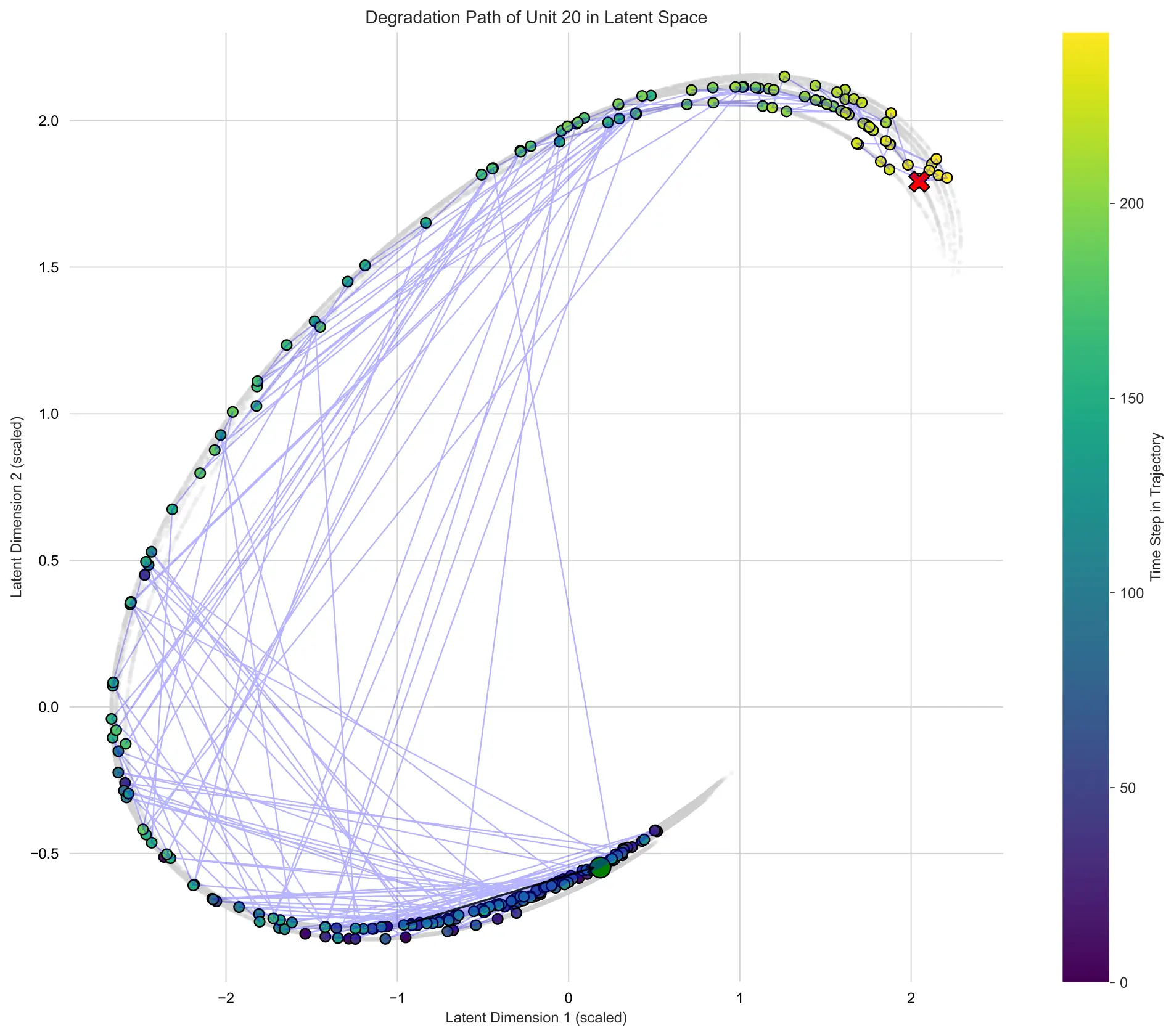
We introduce STEP, a method that learns to arrange sensor data on a kind of compass. Each moment of a machine’s life becomes a point, and its progression toward failure reads as an angle turning from “healthy” to “worn out”, without anyone labelling intermediate stages.
On engine and battery benchmarks, this compass predicts remaining lifetime about as well as specialised models while showing where the machine stands, a step toward maintenance tools engineers can inspect and trust.
Abstract
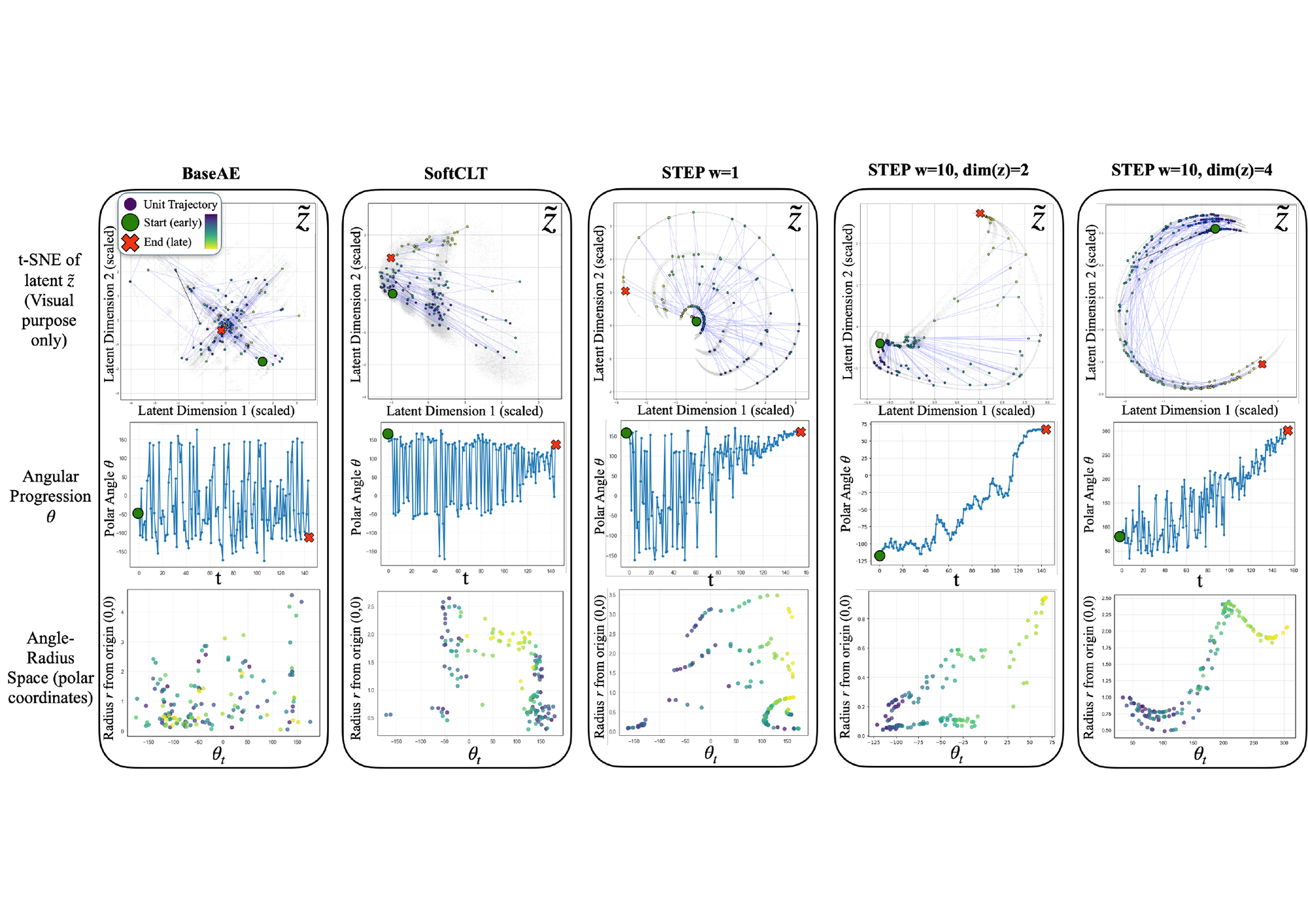
We present a novel method for learning structured representations of progressive time series, that is, data capturing irreversible state transitions such as degradation or task completion. Our approach uses a self-supervised contrastive objective to learn a low-dimensional latent space in which each observation becomes a point on a manifold anchored between two fixed orthogonal prototype vectors, and a trajectory becomes a path across that manifold. From this structure we read a latent compass, the polar coordinates (θ, r) of the latent vector, in which θ tracks the progression of the underlying state (e.g., from healthy to failed) and r exposes residual, non-progression structure, without a supervised progression target. We evaluate the approach on industrial degradation and robotic tasks, validating three key capabilities: (1) end-state prediction, (2) health indicators that track the degradation state, and (3) phase separation. Our method is competitive with or improves over black-box counterparts while exposing the progression through a fixed set of coordinates. A simple linear regressor on top of the learned coordinates is competitive with deep architectures, quantitative evidence that the underlying state is encoded in a geometrically accessible form.
How it works
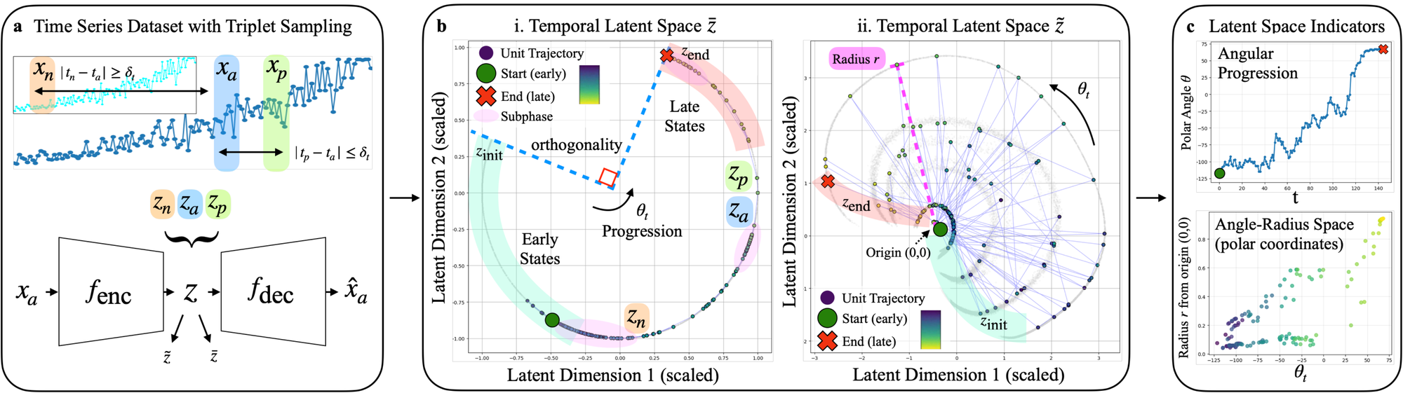
STEP trains an autoencoder with three terms. A cosine triplet loss orders observations along each trajectory, so that nearby moments end up close and distant health states end up apart. A prototype term softly anchors the first and last windows of every training trajectory to two fixed orthogonal vectors, which gives all trajectories a shared reference frame. A reconstruction term keeps the latent informative.
Health indicators are then read straight from this geometry, with no separate progression model. The latent compass gives an angle θ that moves from the start prototype to the end prototype, and a radius r that carries the remaining structure. A full-dimensional Mahalanobis readout gives a quantitative health indicator.
Losses
STEP trains an encoder f_enc and a deliberately small MLP decoder f_dec with three terms combined by scalars (λ1, λ2, λ3).
(1) Contrastive ordering. A cosine triplet loss orders observations along each trajectory. For a triplet (xa, xp, xn) with latent codes (za, zp, zn) and margin m:
Positives share the same unit with |tp − ta| ≤ δt; negatives come from the same unit with |tn − ta| ≥ δt or from a different unit (sampled across coarse remaining-life bands). Since cos(za, zp) = cos(θap), the loss encourages θap < θan, ordering embeddings angularly along the trajectory.
(2) Reconstruction. A small MLP decoder keeps the latent informative (a high-capacity decoder could bypass the latent structure):
(3) Prototype anchoring. Two fixed orthogonal vectors zinit = e1 and zend = e2 give the manifold a shared reference frame. The first k and last k windows of each training trajectory (Xinit, Xend) are softly pulled toward them:
The pull is a soft expectation, leaving slack for unit-level variability (initial-wear spread, radial direction). Anchoring matters when trajectories span heterogeneous regimes: removing it degrades FD004 from 12.10 to 19.01 RMSE.
Full objective.
Readouts. At inference the latent compass uses the two anchor coordinates:
A full-dimensional Mahalanobis readout from the healthy state provides a quantitative health indicator:
What the latent space looks like
The angle follows health, not the clock
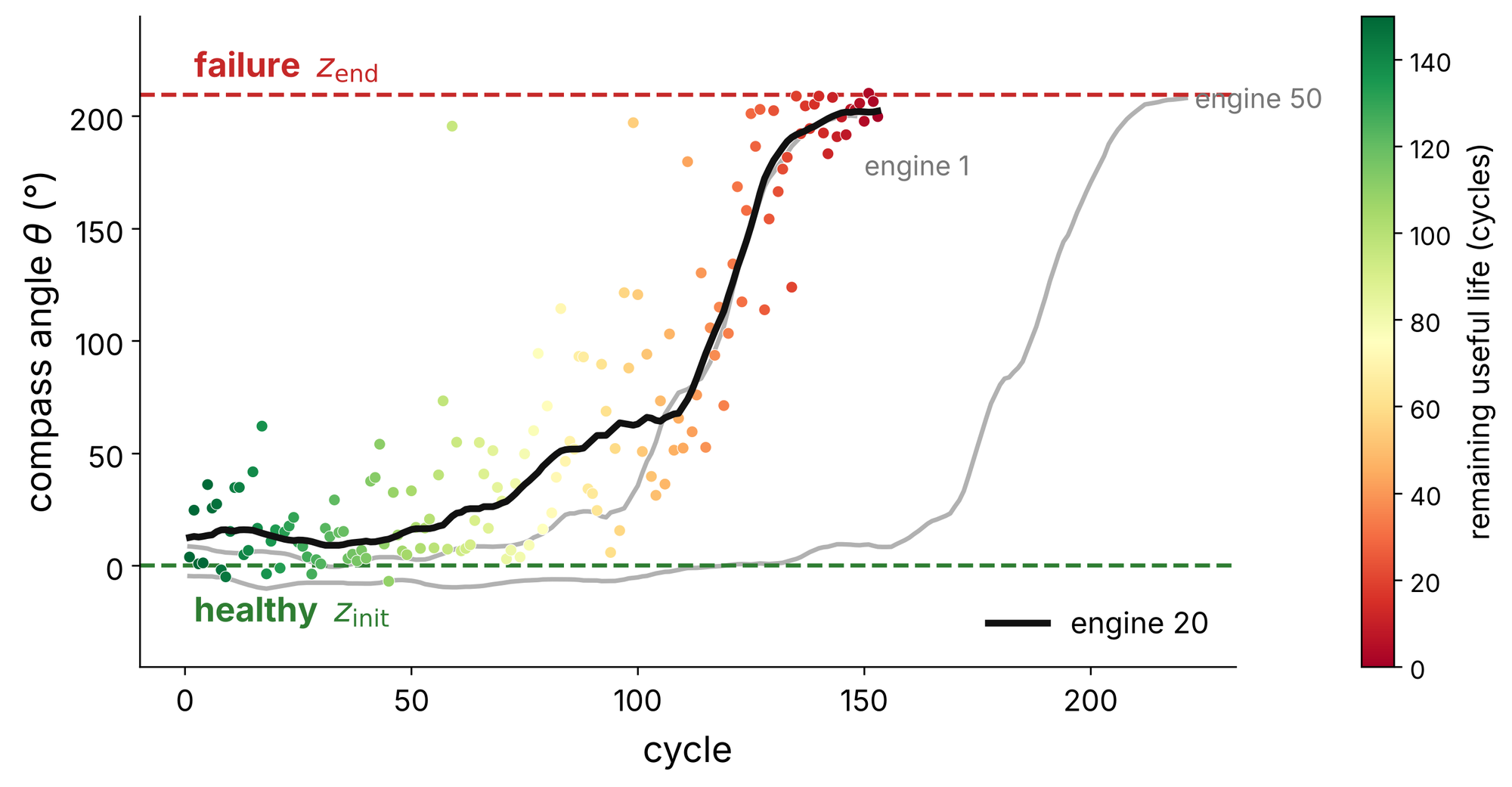
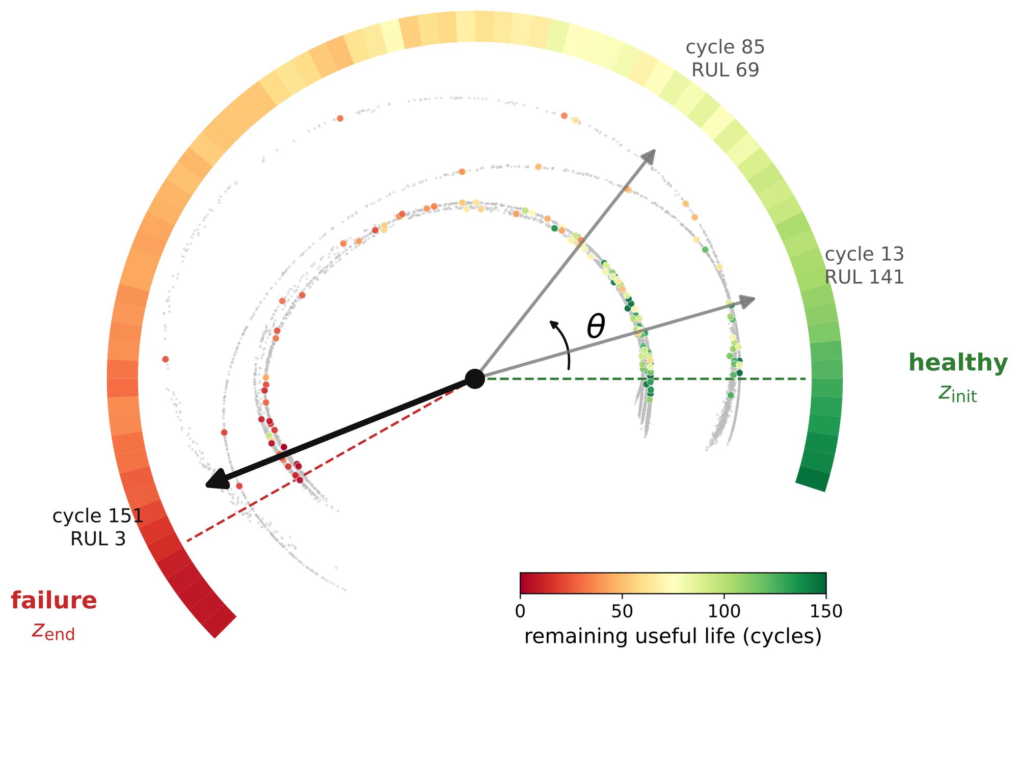
The compass angle over an engine’s life. θ rises with degradation rather than elapsed time. Engine 50 lives longer and turns later.
On held-out engines, the angle carries remaining-life information beyond the number of elapsed cycles. It also ignores the operating regime. A classifier recovers the operating condition from STEP’s angle only at chance level (0.17, against 0.52 for the same backbone trained for reconstruction), while the condition stays readable from the rest of the latent (0.97). STEP moves operating information off the progression axis instead of discarding it.
Results
(same backbone with AE: 0.35–0.46)
(best classical indicator: 0.97)
(reconstruction alone: 9.4)
C-MAPSS remaining useful life, RMSE (lower is better, mean over 5 seeds):
| Model | HI | FD001 | FD002 | FD003 | FD004 |
|---|---|---|---|---|---|
| Published baselines (supervised unless noted) | |||||
| MLP (Zheng et al., 2017) | 37.56 | 80.03 | 37.39 | 77.37 | |
| SVR (Zheng et al., 2017) | 20.96 | 42.00 | 21.05 | 45.35 | |
| RVR (Zheng et al., 2017) | 23.80 | 31.30 | 22.37 | 34.34 | |
| CNN (Zheng et al., 2017) | 18.45 | 30.29 | 19.82 | 29.16 | |
| SSL (Listou Ellefsen et al., 2019) | 12.56 | 22.73 | 12.10 | 22.66 | |
| CNN-LSTM (Peng et al., 2021) | 11.17 | – | 9.99 | – | |
| MS-DCNN (Li et al., 2020) | 11.44 | 19.35 | 11.67 | 22.22 | |
| VAE + RNN (Costa & Sánchez, 2022) | 11.44 | 24.12 | 14.88 | 26.54 | |
| MLE4X + CCF (Pillai & Vadakkepat, 2021) | 11.57 | 18.84 | 11.83 | 20.78 | |
| RVE (Costa & Sánchez, 2022) | 13.42 | 14.92 | 12.51 | 16.37 | |
| Prob. CNN (De Pater & Mitici, 2022) | 12.42 | 13.72 | 12.16 | 15.95 | |
| Wang et al. (2025) | ✓ | – | – | – | 15.42 |
| I-GLIDE (Thil et al., 2025)† | ✓ | 9.47 | 16.18 | 8.29 | 12.32 |
| Same backbone, different objective (our runs, 5 seeds) | |||||
| Tr.AE z=32 (reconstruction only) | 17.15 ± 0.18 | 18.13 ± 0.21 | 20.72 ± 1.41 | 20.76 ± 0.68 | |
| Tr.SoftCLT z=32 | 15.50 ± 0.61 | 19.73 ± 1.25 | 14.87 ± 1.06 | 23.09 ± 2.08 | |
| STEP (ours) | |||||
| Tr.STEP z=2 | ✓ | 13.18 ± 0.79 | 12.13 ± 0.10 | 13.30 ± 0.46 | 15.31 ± 0.84 |
| Tr.STEP z=4 | ✓ | 13.12 ± 0.23 | 11.78 ± 0.40 | 12.89 ± 0.73 | 13.31 ± 0.32 |
| Tr.STEP z=32 (transformer head) | ✓ | 13.27 ± 0.38 | 11.57 ± 0.34 | 12.66 ± 0.51 | 13.13 ± 0.69 |
| LR.STEP z=32 (linear head) | ✓ | 13.09 ± 0.42 | 11.44 ± 0.04 | 12.48 ± 0.48 | 13.26 ± 0.39 |
A plain linear regression on STEP’s coordinates matches the transformer head, showing that the state is linearly accessible in the representation.
Beyond degradation: robot task phases
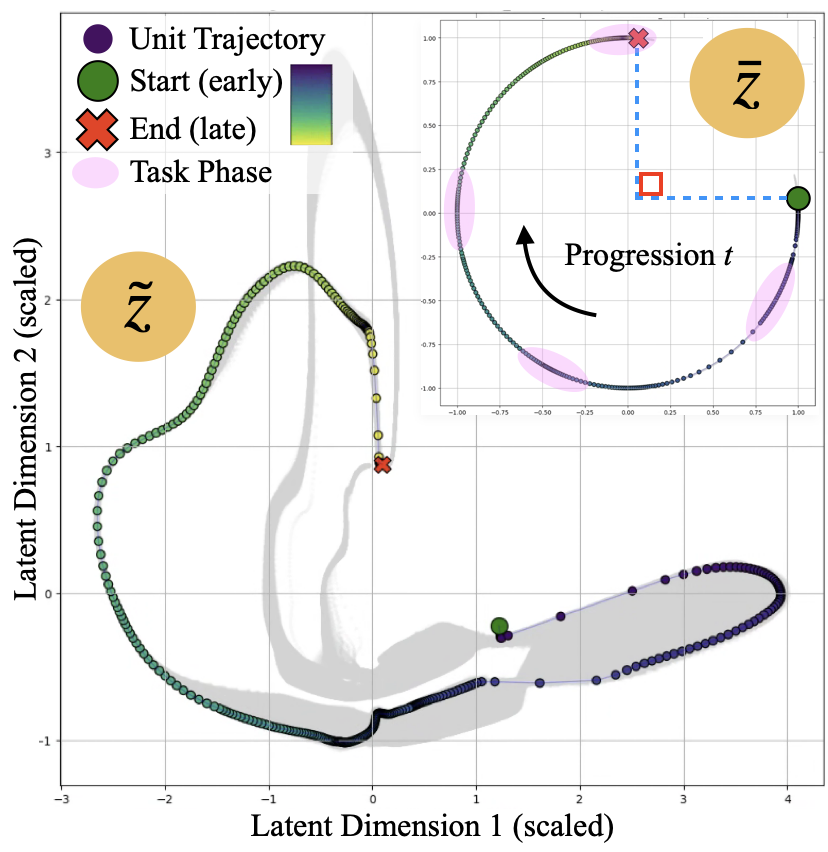
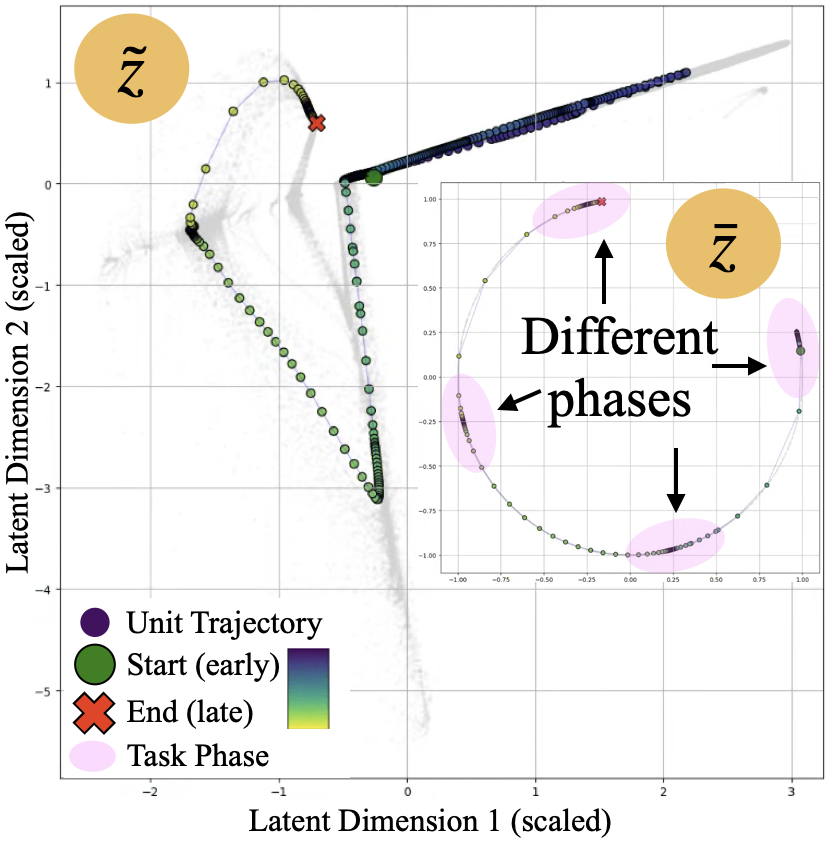
On robotic manipulation episodes (NVIDIA GR00T and LeRobot), the same geometry groups episodes into task phases (locating, grabbing, moving, placing) without annotation. Qualitative.
Limitations
STEP assumes the underlying state does not go back, so maintenance and other reversible transitions are out of scope. It trains on complete run-to-failure trajectories, and it does not model how control inputs change the degradation rate.
Citation
@inproceedings{thil2026step,
  title     = {{STEP}: Learning STructured Embeddings for Progressive Time Series},
  author    = {Thil, Lucas and Read, Jesse and Kaddah, Rim and Doquet, Guillaume},
  booktitle = {Advances in Neural Information Processing Systems (NeurIPS)},
  year      = {2026}
}
Code: github.com/LucasStill/STEP. Paper: NeurIPS 2026. arXiv: 2605.31061. Poster will be added after the conference.